Visualizing Fixation Patterns#
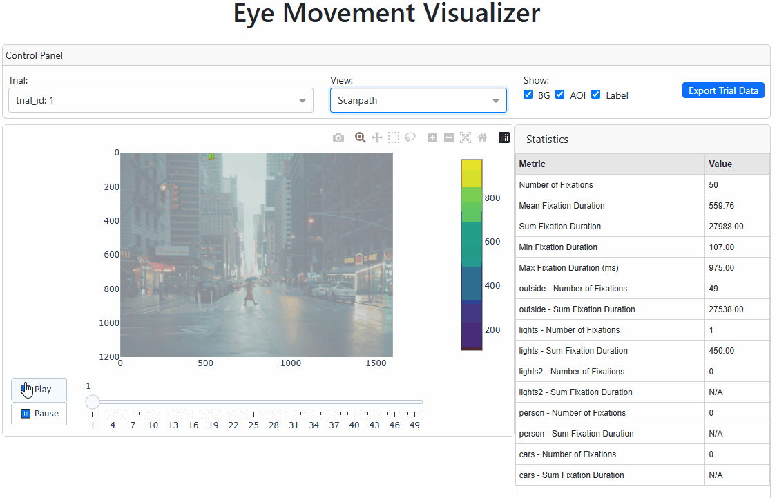
The FixationViewer#
Overview
The FixationViewer provides three visualizations:
A playback of scanpath
A fixation density map (i.e., heatmap)
An areas-of-interest map
It also shows some basic fixation measures, such as fixation count and duration.
FixationViewer should come in handy when you want to get a first impression of eye movement patterns during a particular trial.
To demonstrate how FixationViewer works, let’s first generate some fake data:
import numpy as np
import pandas as pd
import pupeyes as pe

# generate some fake fixation data
screen_dims = (1600, 1200) # width, height
pics = ['street1.jpg', 'street2.jpg']
x = np.random.randint(0, screen_dims[0], size=100)
y = np.random.randint(0, screen_dims[1], size=100)
duration = np.random.randint(100, 1000, size=100)
stimuli = ['street1.jpg'] * 50 + ['street2.jpg'] * 50
trial_id = [1] * 50 + [2] * 50

fixation_data = pd.DataFrame({'x': x, 'y': y, 'duration': duration, 'stimuli': stimuli, 'trial_id': trial_id})
fixation_data
| x | y | duration | stimuli | trial_id | |
|---|---|---|---|---|---|
| 0 | 1362 | 783 | 512 | street1.jpg | 1 |
| 1 | 1012 | 1149 | 431 | street1.jpg | 1 |
| 2 | 1002 | 928 | 818 | street1.jpg | 1 |
| 3 | 1060 | 1012 | 266 | street1.jpg | 1 |
| 4 | 167 | 462 | 801 | street1.jpg | 1 |
| ... | ... | ... | ... | ... | ... |
| 95 | 501 | 843 | 955 | street2.jpg | 2 |
| 96 | 510 | 789 | 142 | street2.jpg | 2 |
| 97 | 1129 | 873 | 448 | street2.jpg | 2 |
| 98 | 1438 | 418 | 898 | street2.jpg | 2 |
| 99 | 1574 | 519 | 727 | street2.jpg | 2 |
100 rows × 5 columns
Note
Note that these columns are not Eyelink-specific. You may export a data file like this from Tobii Pro Lab and it will work with the fixation analyses functions in PupEyes.
The fake data consists of 2 trials, with each trial including 50 fixations on the associated stimulus.
Next, we will define some AOIs. I already did this using the AOIDrawer tool. So I will just load those .json files and format the AOIs in a way that’s supported by FixationViewer.
import json

# load AOIs
with open('assets/street1_aois.json', 'r') as f:
    aois1 = json.load(f)

with open('assets/street2_aois.json', 'r') as f:
    aois2 = json.load(f)

# nested dictionary
aois = {
    'street1.jpg': aois1, # key is the stimulus name in the data
    'street2.jpg': aois2
}
The final step is to initialize FixationViewer by passing the correct arguments.
from pupeyes import FixationViewer

# path that stores my stimulus pictures
pic_path = 'assets/'

# Create visualizer
viz = FixationViewer(
    data=fixation_data,  # your fixation dataframe
    screen_dims = (1600, 1200),
    stimuli_path = pic_path,
    col_mapping={
        'trial_id': 'trial_id',  # List of columns that identify a trial
        'x': 'x',  # x coordinate column name
        'y': 'y',  # y coordinate column name
        'duration': 'duration',  # duration column name
        'stimuli': 'stimuli'  # uncomment if you have stimuli images
    }
)

# Set AOIs if needed
viz.set_aois(aois)

# viz.run()
No timestamp column specified.
Below is an animation of FixationViewer as it runs on my local machine.
Note
The timestamp and duration columns are optional. Some measures will not be displayed, however.
Error
Known Issues Currently, autoscaling and resetting axes do not correctly reset axes for the scanpath plot and the AOI plot.
Static Drawing Tools#
PupEyes also provides several static drawing options using matplotlib.
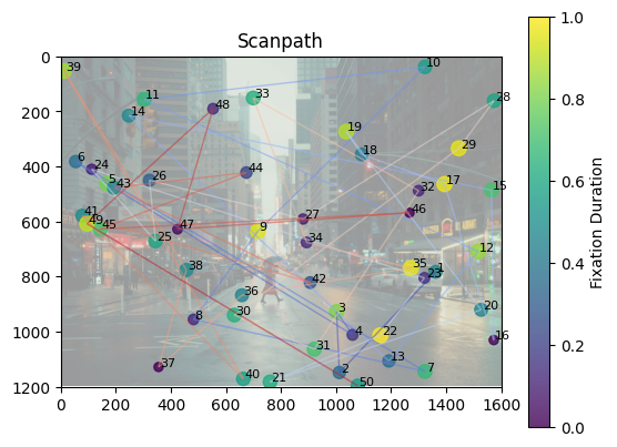
Scanpaths#
from pupeyes import draw_scanpath

plot_data = fixation_data.query('trial_id==1')
path = 'assets/street1.jpg'

draw_scanpath(x=plot_data['x'], y=plot_data['y'], screen_dims=(1600, 1200), durations=plot_data['duration'], background_img=path)
Original size: (6231, 4154) Resized size: (1600, 1200)
(<Figure size 640x480 with 2 Axes>, <Axes: title={'center': 'Scanpath'}>)
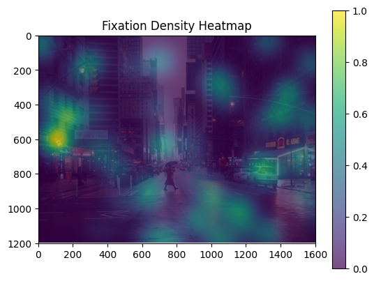
Drawing Heatmap#
from pupeyes import draw_heatmap

draw_heatmap(x=plot_data['x'], y=plot_data['y'], screen_dims=(1600, 1200), durations=plot_data['duration'], background_img=path)
Original size: (6231, 4154) Resized size: (1600, 1200)
(<Figure size 640x480 with 2 Axes>,
 <Axes: title={'center': 'Fixation Density Heatmap'}>)
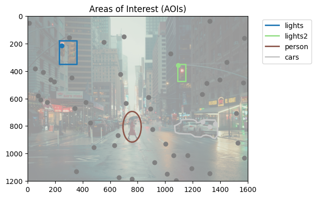
Draw AOIs#
from pupeyes import draw_aois

draw_aois(aois=aois1, x=plot_data['x'], y=plot_data['y'], screen_dims=(1600, 1200), background_img=path)
Original size: (6231, 4154) Resized size: (1600, 1200)
(<Figure size 640x480 with 1 Axes>,
 <Axes: title={'center': 'Areas of Interest (AOIs)'}>)