
Statistical Analysis of Pupil Data#
Overview
PupEyes is designed for preprocessing: preparing your data in an analysis-friendly format so you can perform whatever analyses that you deem appropriate for your research goals. Indeed, there are many ways to analyze pupil size data, and it would be impractical to implement them all. However, to demonstrate how easily you can conduct analyses with preprocessed PupEyes data, we will cover some basic examples:
Using a Predefined Time Window
Plotting Evoked Responses
Cluster-based Permutation Testing
Note
Some analyses in this tutorial require the mne package, a Python library for visualizing and analyzing neurophysiological data. mne is not included as a dependency for PupEyes. For information on how to install, see: https://mne.tools/stable/install/index.html
Example Task#
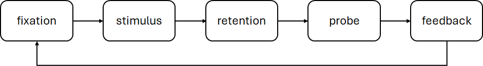
Suppose our example memory task has a within-subject condition called “memory load.” On low-load trials, only 3 letters were presented. On high-load trials, 6 letters were presented. We are interested in whether high-load trials elicit a larger task-evoked pupillary response than low-load trials. This is a common scenario in which task-evoked pupillary responses are compared between the levels of a within-subject factor.
First, let’s generate some fake pupil data for this task.
import pandas as pd
import numpy as np
import matplotlib.pyplot as plt
import pupeyes as pe
from pupeyes.pupil import _generate_pupil_data

%matplotlib inline
data_within =_generate_pupil_data(condition_names=['high load','low load'])

data_within.groupby(['participant', 'condition']).trial.nunique()
participant  condition
P1           high load    10
             low load     10
P2           high load    10
             low load     10
P3           high load    10
             low load     10
P4           high load    10
             low load     10
P5           high load    10
             low load     10
P6           high load    10
             low load     10
Name: trial, dtype: int64
We have generated a pupil dataset for a within-subject design, with 6 participants completing 10 trials in each condition.
Pupil Preprocessing#
Since our focus here is on statistical analyses, I’m going to quickly do preprocessing using a set of default choices and skip diagnostics. For real data, though, this is probably not a good idea unless you know what you are doing. Check out the Pupil Preprocessing tutorial for more information on pupil preprocessing steps.
def my_pipeline(data):
    """This is probably not a good idea for real data.
    """
    # Do preprocessing
    p = pe.PupilProcessor(
        data=data_within,
        trial_identifier=['participant', 'condition', 'trial'],
        x_col = 'x',
        y_col = 'y',
        pupil_col = 'pp',
        time_col = 'trialtime',
        samp_freq = 1000,
        convert_pupil_size=False,
        progress_bar=False
        )\
        .deblink()\
        .artifact_rejection()\
        .smooth()\
        .interpolate(missing_threshold=.4)\
        .baseline_correction(baseline_query='event=="fixation"', baseline_range=[-100, None])

    # Create a final dataset with only valid trials during stimulus presentation
    p.final_data = p.data.query('event=="stimulus"').reset_index(drop=True)

    # Rename the fully preprocessed pupil column to something more manageable
    p.final_data['pp_final'] = p.final_data['pp_db_ar_sm_it_bc']

    # Select only the relevant columns for analysis
    p.final_data = p.final_data[[
        'condition',    # condition
        'participant',  # participant ID
        'trial',        # trial number
        'event',        # event marker
        'trialtime',    # time relative to trial onset
        'x', 'y',       # gaze coordinates
        'pp_final'      # preprocessed pupil size
    ]]

    # Create a timestamp column indicating time since stimulus onset using pandas' groupby-transform routine
    p.final_data['eventtime'] = p.final_data.groupby(['participant','condition','trial'], sort=False).trialtime.transform(lambda x: x - x.iloc[0]) # reset timestamp for each trial

    return p

p = my_pipeline(data_within)
Device: eyelink
Eye-tracker missing value for pupil size is 0. No replacement needed.
Sampling frequency check passed. Sampling rate: 1000Hz
PupilProcessor initialized with 300000 samples
Pupil column: pp, Time column: trialtime, X column: x, Y column: y
Trial identifier: ['participant', 'condition', 'trial'], Number of trials: 120
Running deblink using sampling frequency 1000Hz
✓ Deblinking completed!
  → New column: 'pp_db' (blinks removed)
  → Previous column 'pp' preserved.
  → 0 trial(s) failed.
✓ Artifact rejection completed!
  → New column: 'pp_db_ar' (artifacts removed)
  → Previous column 'pp_db' preserved.
  → 0 trial(s) failed.
✓ Smoothing completed!
  → New column: 'pp_db_ar_sm' (smoothed)
  → Previous column 'pp_db_ar' preserved.
  → 0 trial(s) failed.
✓ Interpolation completed!
  → New column: 'pp_db_ar_sm_it' (interpolated)
  → Previous column 'pp_db_ar_sm' preserved.
  → 0 trial(s) failed.
✓ Baseline correction completed!
  → New column: 'pp_db_ar_sm_it_bc' (baseline corrected)
  → Previous column 'pp_db_ar_sm_it' preserved.
  → 0 trial(s) failed.
# Preview the data
p.final_data.head(5)
| condition | participant | trial | event | trialtime | x | y | pp_final | eventtime | |
|---|---|---|---|---|---|---|---|---|---|
| 0 | low load | P1 | 1 | stimulus | 500 | 942.185932 | 507.713273 | 0.005327 | 0 |
| 1 | low load | P1 | 1 | stimulus | 501 | 996.015392 | 540.323535 | 0.00529 | 1 |
| 2 | low load | P1 | 1 | stimulus | 502 | 941.540018 | 553.377994 | 0.005231 | 2 |
| 3 | low load | P1 | 1 | stimulus | 503 | 968.662738 | 557.507127 | 0.005151 | 3 |
| 4 | low load | P1 | 1 | stimulus | 504 | 956.29782 | 517.937173 | 0.005055 | 4 |
Use a Predefined Time Window#
If you have a (preferably pre-registered) hypothesis for when your task-evoked pupillary response will emerge, you can simply select that time window and compute the mean pupil size within that window.
For example, if we hypothesize that the effect emerges during 600 ms to 1000 ms after stimulus onset:
df_600to1000 = p.final_data.query('eventtime > 600 & eventtime < 1000').groupby(['participant','condition','trial']).pp_final.mean()
df_600to1000
/tmp/ipykernel_896/1065545117.py:1: RuntimeWarning: Engine has switched to 'python' because numexpr does not support extension array dtypes. Please set your engine to python manually.
  df_600to1000 = p.final_data.query('eventtime > 600 & eventtime < 1000').groupby(['participant','condition','trial']).pp_final.mean()
participant  condition  trial
P1           high load  3        0.411048
                        5       -0.001736
                        8       -0.004048
                        9       -0.006161
                        11       0.865803
                                   ...
P6           low load   13        0.42528
                        15      -0.002152
                        16       0.292533
                        19       0.309909
                        20       0.094568
Name: pp_final, Length: 120, dtype: Float64
From now on, mean pupil sizes can be analyzed in the same way as response times (RTs).
Plot Evoked Response#
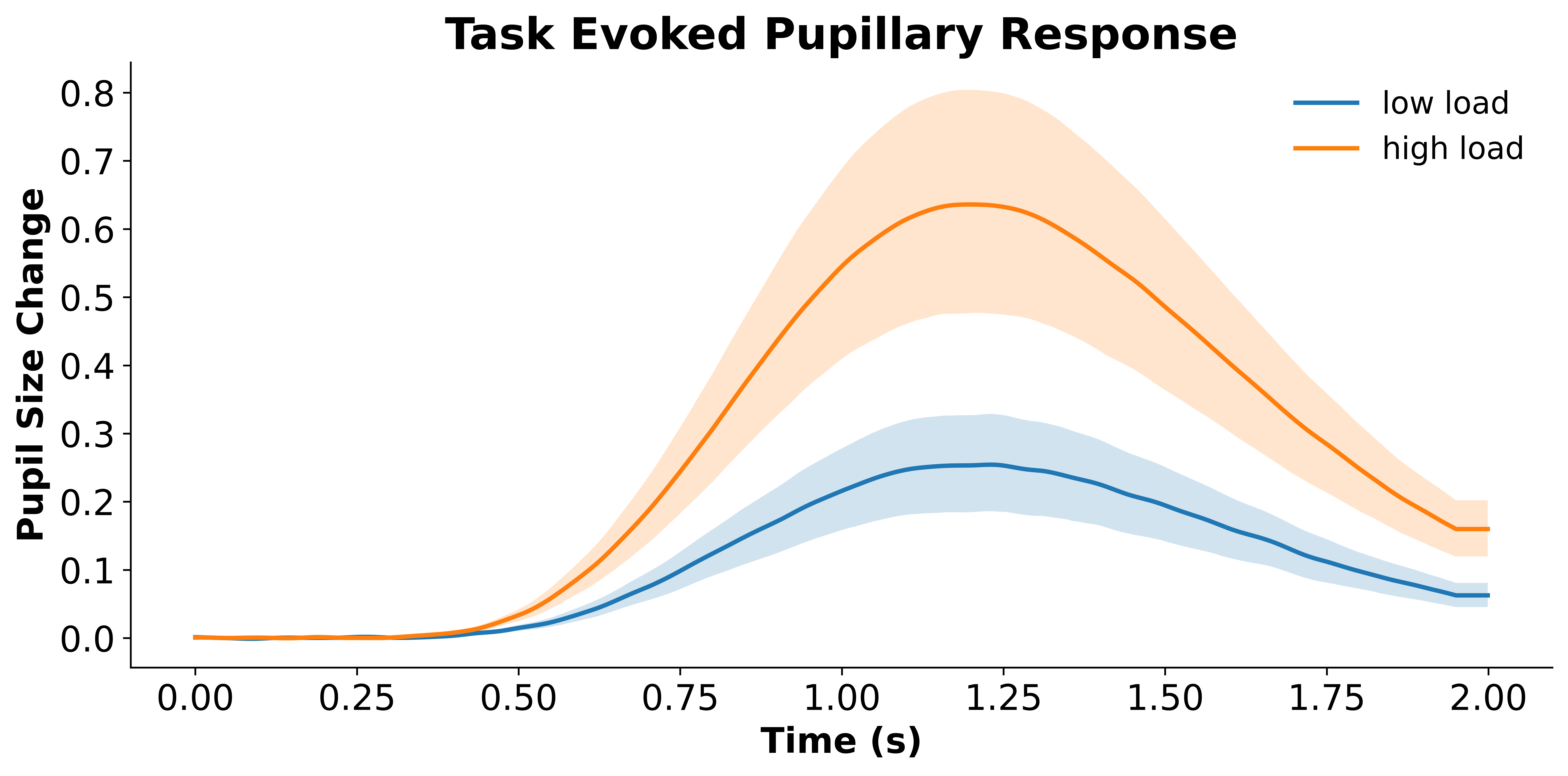
Oftentimes we do not have a hypothesis about when an effect should emerge. Even if we do, it is always nice to have a plot showing the entire evoked response. PupEyes has a built-in method, .plot_evoked(), to plot evoked responses. For example, the plot below shows grand average pupillary responses and their associated confidence bands for conditions A and B.
data_grandavg, (fig, ax) = p.plot_evoked(
    data='final_data',
    condition='condition',
    pupil_col='pp_final',
    error='ci',  # ci requires mne
)
Data will be padded to minimum length: 2000 samples
Condition {'condition': 'low load'}: Computing average from 60 trials
Condition {'condition': 'high load'}: Computing average from 60 trials
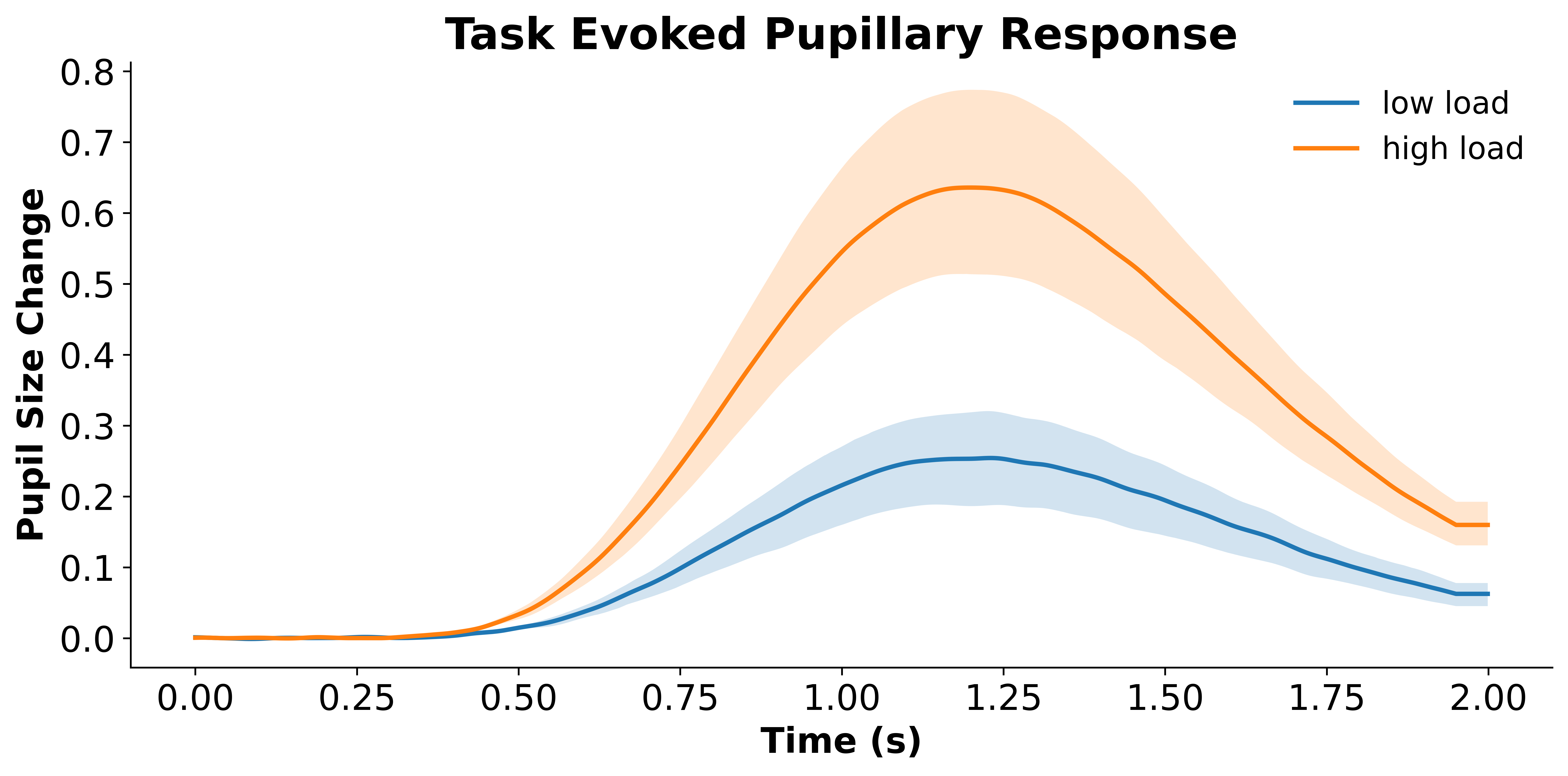
You can also aggregate the data before plotting. For example, specifying agg_by='participant' will compute an averaged trace for each participant first and then plot the data based on participant-level traces, much like computing a mean RT for each participant and then plotting the average RT across participants.
data_sub_level, (fig, ax) = p.plot_evoked(
    data='final_data',
    agg_by='participant', # aggregate by participant
    condition='condition',
    pupil_col='pp_final',
    error='ci')
Data will be padded to minimum length: 2000 samples
Condition {'condition': 'low load'}: Computing average from 6 ['participant'] means
Condition {'condition': 'high load'}: Computing average from 6 ['participant'] means
You might have noticed that .plot_evoked() not only returns the plot but also the data. The returned data will be discussed in the next section.
Cluster-based Permutation Testing#
Does condition A elicit a statistically different pupillary response compared to condition B? Pupil data easily consists of thousands of data points, which creates a multiple-comparison problem: If a statistical test is performed for every time point, it will easily end up having thousands of tests. Simply performing a Bonferroni correction seems too strict and limits statistical power. Therefore, it is common practice to conduct cluster-based permutation testing to determine whether the data is indistinguishable from chance (or from another condition).
The .plot_evoked() method not only returns the plot but also the data that the plot is based on. For example, data_sub_level is a dictionary with the two conditions (A and B) as keys. For each condition, the returned data is a 6*2000 array because we have 6 subjects with each subject having 2000 data points (i.e., 2000 ms with 1000 Hz sampling rate). Note that each data point is averaged across all trials within that participant.
data_sub_level
{'low load': array([[ 0.00255182,  0.0025651 ,  0.00257478, ...,  0.07409407,
          0.07409407,  0.07409407],
        [ 0.0003461 ,  0.00029606,  0.00023656, ...,  0.07115299,
          0.07115299,  0.07115299],
        [ 0.00027453,  0.00028043,  0.00028342, ...,  0.05610489,
          0.05610489,  0.05610489],
        [ 0.00298366,  0.00301351,  0.00303881, ...,  0.05059733,
          0.05059733,  0.05059733],
        [ 0.00334893,  0.00345346,  0.00355353, ...,  0.02946476,
          0.02946476,  0.02946476],
        [-0.00154587, -0.00168687, -0.00182268, ...,  0.09462795,
          0.09462795,  0.09462795]], shape=(6, 2000)),
 'high load': array([[-0.00138876, -0.00136447, -0.00134291, ...,  0.14159611,
          0.14159611,  0.14159611],
        [-0.00074718, -0.00073473, -0.00071962, ...,  0.18119371,
          0.18119371,  0.18119371],
        [ 0.00052207,  0.0005919 ,  0.00065841, ...,  0.13458076,
          0.13458076,  0.13458076],
        [ 0.00242086,  0.00239059,  0.002354  , ...,  0.24402741,
          0.24402741,  0.24402741],
        [ 0.0017825 ,  0.00186673,  0.00195012, ...,  0.1170127 ,
          0.1170127 ,  0.1170127 ],
        [ 0.00180697,  0.0018087 ,  0.00180812, ...,  0.14113933,
          0.14113933,  0.14113933]], shape=(6, 2000))}
We can pass the difference between condition A and B to permutation_cluster_1samp_test for a cluster-based permutation t-test. Note that a one-sample t-test on the difference score in a within-subject design is essentially the same as a paired t-test.
The tests are completely handled by the mne package.
import mne.stats as ms

# Cluster-based permutation test on the difference between conditions A - B
T_obs, clusters, cluster_p_values, H0 = ms.permutation_cluster_1samp_test(
    data_sub_level['high load'] - data_sub_level['low load'],
    threshold=None, # if None, then mne will use critical t when p = 0.5
    tail=0, # two-tailed test
    out_type="mask",
)
Using a threshold of 2.570582
stat_fun(H1): min=-0.9460307251398432 max=4.67045648456268
Running initial clustering …
Found 1 cluster
# range for each cluster
clusters
[(slice(434, 2000, None),)]
# p value for each cluster
cluster_p_values
array([0.03125])
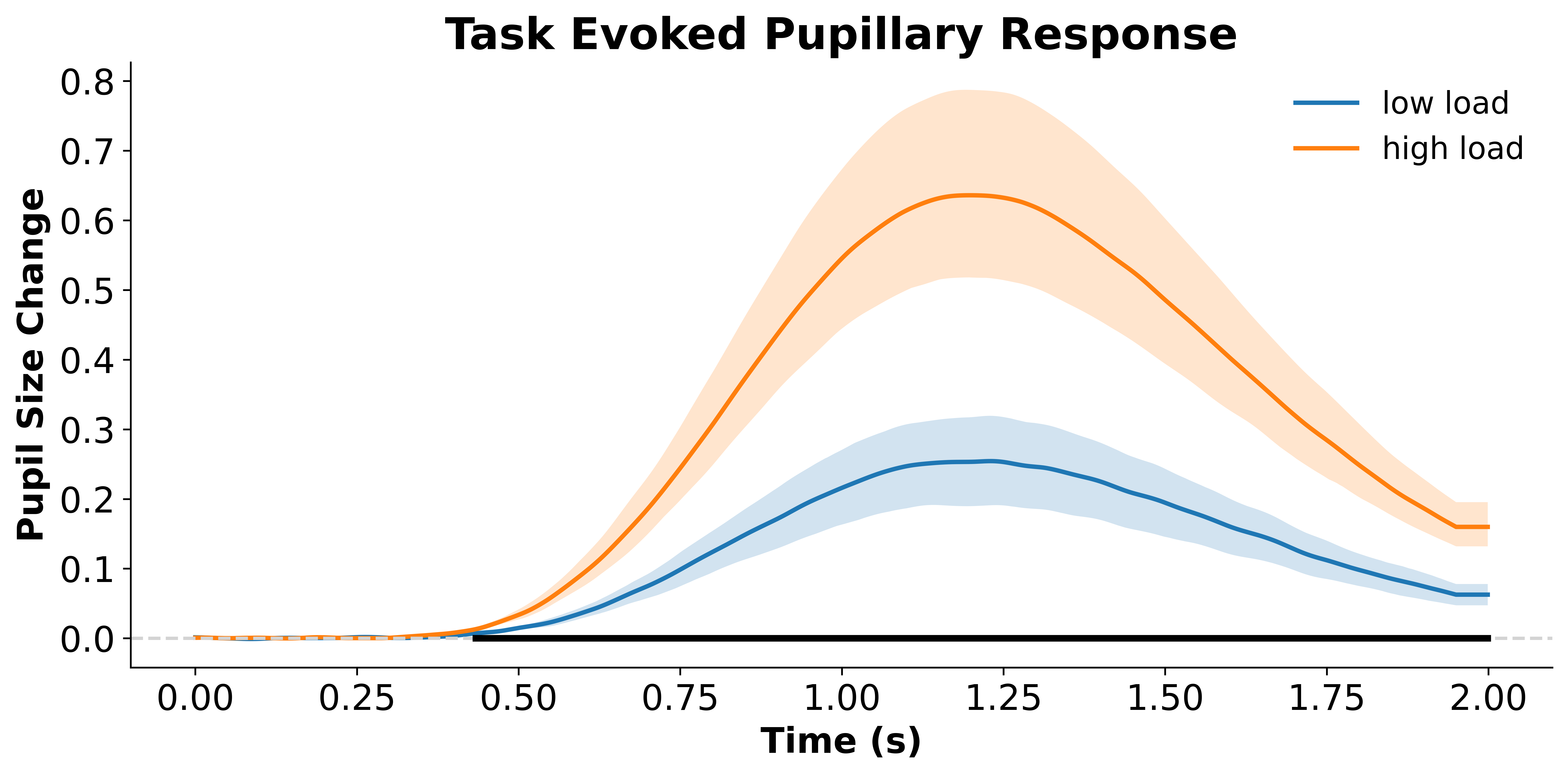
The results indicate that condition A elicits a statistically different pupillary response compared to condition B.
We can visualize the found clusters on our original plot:
data_sub_level, (fig, ax) = p.plot_evoked(
    data='final_data',
    agg_by='participant', # aggregate by participant
    condition='condition',
    pupil_col='pp_final',
    error='ci')

# baseline
ax.axhline(0, color='lightgrey', linestyle='--')

# get timestamps
t = np.arange(data_sub_level['high load'].shape[1]) / 1000 # divided by sampling rate to get time vector

# plot clusters
for i, cluster in enumerate(clusters):
    if cluster_p_values[i] < .05: # check cluster p value
        ax.plot(t[cluster], [0]*len(t[cluster]), color='black', linewidth=3)
Data will be padded to minimum length: 2000 samples
Condition {'condition': 'low load'}: Computing average from 6 ['participant'] means
Condition {'condition': 'high load'}: Computing average from 6 ['participant'] means
Q & A#
Between-subject Comparison?#
If you want to compare, say, pupil response between young vs. older adults, then you will have two arrays of data instead of a single array of difference scores. You can use the permutation_cluster_test() provided in mne, which performs a one-way ANOVA instead of an independent-sample t-test.
F_obs, clusters, cluster_p_values, H0 = ms.permutation_cluster_test(
    [data['Young'], data['Old']], # pass both conditions as a list
    threshold=None, # if None, then mne will use critical F when p = 0.5
    out_type="mask",
)
See also
How not to interpret the results: https://www.fieldtriptoolbox.org/faq/stats/clusterstats_interpretation/
mneAPI Reference: https://mne.tools/stable/generated/mne.stats.permutation_cluster_1samp_test.html