Pupil Preprocessing

Pupil Preprocessing#

Overview

Pupil preprocessing in PupEyes comes down to:

Initialize PupilProcessor with required information.
Do preprocessing using a pipeline of methods.
Quality check using interactive tools.
Finalize: Exclude trials, finalize data, and save results.

Let’s keep using the memory task as an example: on each trial, we ask participants to memorize some letters (e.g., XFABWS), and after a while, we present a probe letter (e.g., A) and ask if this letter belongs to the presented letters.

As a recap, the trial flow looks like this:

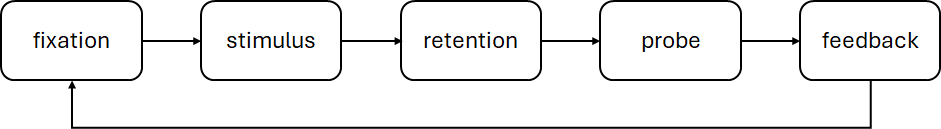
Our example data consists of four participants completing 10 trials of the task.

Read Data#

import pandas as pd
import pupeyes as pe

Here we will use the formatted data from the Read Data tutorial. The data contains gaze sample of four subjects each completing 10 trials.

# load data
samples = pd.read_csv('data/samples.csv')

# select only useful columns
samples = samples[['participant','block','trial','event','trialtime','x','y','pp']]

samples

	participant	block	trial	event	trialtime	x	y	pp
0	sub004	A	1	fixation	0	0.0	0.0	0
1	sub004	A	1	fixation	1	0.0	0.0	0
2	sub004	A	1	fixation	2	0.0	0.0	0
3	sub004	A	1	fixation	3	0.0	0.0	0
4	sub004	A	1	fixation	4	0.0	0.0	0
...	...	...	...	...	...	...	...	...
679960	sub001	A	10	feedback	22927	839.7	484.5	5060
679961	sub001	A	10	feedback	22928	839.7	484.4	5062
679962	sub001	A	10	feedback	22929	839.6	485.5	5064
679963	sub001	A	10	feedback	22930	839.5	486.8	5065
679964	sub001	A	10	feedback	22931	839.6	488.2	5066

679965 rows × 8 columns

Note

Although we used Eyelink data here, note that data from any eye-tracker can work as long as it is formatted as the above. Specifically, it needs to have column(s) that identifies an unique trial, a timestamp column, x & y coordinates, and pupil size. You can get the information from most eye-trackers. The “event” column indicates different parts within a single trial and is not strictly needed.

Check the API reference for more information.

Inititalize PupilProcessor#

The first step of pupil processing is to initiate the PupilProcessor. We simply feed the following information:

p = pe.PupilProcessor(
    data=samples, # pass your data
    trial_identifier=['participant', 'block', 'trial'], # column(s) that disambiguate one trial from another in your data
    x_col = 'x',
    y_col = 'y',
    pupil_col = 'pp',
    time_col = 'trialtime',
    samp_freq = 1000, # Hz
    convert_pupil_size=False, # see note
    progress_bar=False
    )

Device: eyelink
Eye-tracker missing value for pupil size is 0. No replacement needed.

Sampling frequency check passed. Sampling rate: 1000Hz
PupilProcessor initialized with 679965 samples
Pupil column: pp, Time column: trialtime, X column: x, Y column: y
Trial identifier: ['participant', 'block', 'trial'], Number of trials: 40

p.data

	participant	block	trial	event	trialtime	x	y	pp
0	sub004	A	1	fixation	0	0.0	0.0	0
1	sub004	A	1	fixation	1	0.0	0.0	0
2	sub004	A	1	fixation	2	0.0	0.0	0
3	sub004	A	1	fixation	3	0.0	0.0	0
4	sub004	A	1	fixation	4	0.0	0.0	0
...	...	...	...	...	...	...	...	...
679960	sub001	A	10	feedback	22927	839.7	484.5	5060
679961	sub001	A	10	feedback	22928	839.7	484.4	5062
679962	sub001	A	10	feedback	22929	839.6	485.5	5064
679963	sub001	A	10	feedback	22930	839.5	486.8	5065
679964	sub001	A	10	feedback	22931	839.6	488.2	5066

679965 rows × 8 columns

Note

Eyelink records pupil size in an arbitrary unit (AREA or DIAMETER, depending on your system setting). These arbitrary pupil sizes can be converted to millimeters by calibrating them against an artificial eye. PupEyes can automatically do this for you if you provide the required information. For example: convert_pupil_size=True, artificial_d=5, artificial_size=5663, recording_unit='diameter'. This should work with other eye-trackers if you know it is recording an area or a diameter. Refer to the API for more information.

Deblink#

Deblinking is finding samples during blinks and setting them as missing. This is usually the first step of pupil preprocessing because blinks cause artificial changes in pupil size.

Running deblinking is just one line of code:

p = p.deblink()

Running deblink using sampling frequency 1000Hz

✓ Deblinking completed!
  → New column: 'pp_db' (blinks removed)
  → Previous column 'pp' preserved.
  → 0 trial(s) failed.

Note

Eyelink automatically detects blinks but its algorithm tends to be over-conservative in marking samples as blinks. For example, it does not account for the opening and closing of eyelids, during which pupil size changes rapidly and can also cause large distortions in the data. Therefore, PupEyes uses a novel algorithm introduced by Hershman et al. (2018) for deblinking, which, based on my own experience, does a better job than Eyelink’s default. So, these detected blinks may be different from those you get from EyelinkReader.get_blinks() as `.get_blinks() just extracts those automatically detected by Eyelink.

For every preprocessing step, PupEyes add a new column with a suffix to store the new data, while preserving the existing data. Here, pp_db is the deblinked data.

 # show the first 5 rows
p.data.head(5)

	participant	block	trial	event	trialtime	pp_db
0	sub004	A	1	fixation	0	<NA>
1	sub004	A	1	fixation	1	<NA>
2	sub004	A	1	fixation	2	<NA>
3	sub004	A	1	fixation	3	<NA>
4	sub004	A	1	fixation	4	<NA>

PupEyes also has a .summary() method that summarizes each preprocessing step. Here, we only have a summary for deblinking. But as we perform more preprocessing, more columns will be added to the summary data. We will revisit .summary() later.

# show the first 5 trials
p.summary().head(5)

	participant	block	trial	n_samples	run_deblink	pct_deblink
0	sub004	A	1	23115	True	0.042743
1	sub004	A	2	23166	True	0.248468
2	sub004	A	3	12197	True	0.169796
3	sub004	A	4	10916	True	0.19705
4	sub004	A	5	22768	True	0.157809

Downsampling (Optional)#

Many modern eye-trackers record pupil data at a very high sampling rate such as 1000 Hz. This may be an overkill given how slow pupillary responses usually are. To speed up processing, it may be desirable to downsample your data to a lower frequency. It is important to note that certain preprocessing steps, such as deblinking, would benefit from high-frequency data. So you may want to downsample after blinks are removed.

Here we create a copy of the original PupilProcessor to demonstrate downsampling. The latter steps are performed without downsampling.

p_downsampled = p.copy() # create a copy of the original instance
p_downsampled.downsample(target_samp_freq=100) # downsample to 100 Hz

Sampling frequency check passed. Sampling rate: 100Hz
✓ Downsampling completed!
  → New sampling frequency: 100 Hz
  → 0 trial(s) failed.

<pupeyes.pupil.PupilProcessor at 0x7749df3193a0>

As the trialtime column indicates the data are now at 100 Hz:

p_downsampled.data.head(5)

	participant	block	trial	event	trialtime	pp_db
0	sub004	A	1	fixation	0	<NA>
1	sub004	A	1	fixation	10	<NA>
2	sub004	A	1	fixation	20	<NA>
3	sub004	A	1	fixation	30	<NA>
4	sub004	A	1	fixation	40	<NA>

PupEyes also has an upsample method in case you want to align your data with those recorded from other devices that have a higher sampling rate. More info: API Reference.

Artifact Rejection#

Besides blinking, many other factors can introduce pupil size artifacts (e.g., head movement). Therefore, it is a good idea to do further cleaning after deblinking.

PupEyes implements an artifact_rejection() method for this purpose. The user can choose to remove artifacts based on one or both of these methods:

Rapid change in pupil size. This method identifies rapid changes in pupil size. The speed threshold is set as a constant speed_n * the Median Absolute Deviation (MAD) of pupil speeds. The default value of speed_n = 16. This method is recommended here, here, and here.
Extreme pupil sizes. This method identifies extreme pupil sizes based on z-scores while protecting stable data from being removed, based on an implementation here.

The default is to use both methods but the user may choose to use only one with method='speed' or method='zscore'.

p = p.artifact_rejection()

✓ Artifact rejection completed!
  → New column: 'pp_db_ar' (artifacts removed)
  → Previous column 'pp_db' preserved.
  → 0 trial(s) failed.

Filter Gaze Positions#

Many pupillometry experiments restrict eye movements for a good reason: to minimize the pupil foreshortening error, that is, size artifacts introduced when the eyeballs rotate away from the camera. Therefore, it may be a good idea to remove samples that deviate too much from the screen center. PupEyes provides a filter_position method for this purpose.

You just need to provide a list of vertices that define your “good” region. For this example, we will set the region to be the screen. Any samples looking outside of the screen will be removed.

# vertices are in Eyelink coordinates (top-left corner (0,0)); last point to close the polygon
vertices = [(0,0), (0, 1080), (1920, 1080), (1920, 0), (0,0)] 
p = p.filter_position(vertices=vertices)

✓ Gaze spatial filtering completed!
  → New column: 'pp_db_ar_xy' (gaze filtered)
  → Previous column 'pp_db_ar' preserved.
  → 0 trial(s) failed.

Smooth Data#

Even with a perfect participant, eye-trackers themselves produce high-frequency noise that should be smoothed out before analysis. There are many ways to smooth the data. PupEyes provides three options:

Hanning window (method='hann')
Rolling mean (method='rollingmean')
Butterworth low-pass filter (method='butter'; requires non-missing data, so interpolate data first)

Here, we will use the Hanning window with a window size of 100 (i.e., 100 samples), which is the default option.

p = p.smooth()

✓ Smoothing completed!
  → New column: 'pp_db_ar_xy_sm' (smoothed)
  → Previous column 'pp_db_ar_xy' preserved.
  → 0 trial(s) failed.

Check Missing Data#

So far we have set pupil size values to missing for various reasons. It is a good idea to check for missingness at this point to get a sense data quality.

p = p.check_missing() # default is the lastest pupil size column

✓ Missing values checked!
  → 0 trial(s) failed.

p.summary().head(5)

	participant	block	trial	n_samples	run_deblink	pct_deblink	run_speed	pct_speed	run_size	run_gaze_filter	pct_gaze_filter	avg_gaze_x	avg_gaze_y	run_smooth	run_check_missing	missing
0	sub004	A	1	23115	True	0.042743	True	0.000692	True	True	0.001298	932.023893	592.014834	True	True	0.061302
1	sub004	A	2	23166	True	0.248468	True	0.001597	True	True	0.03203	975.807543	604.144581	True	True	0.340456
2	sub004	A	3	12197	True	0.169796	True	0.002378	True	True	0.018775	955.872528	597.951776	True	True	0.250143
3	sub004	A	4	10916	True	0.19705	True	0.002657	True	True	0.066141	954.471826	580.816997	True	True	0.323837
4	sub004	A	5	22768	True	0.157809	True	0.001976	True	True	0.022356	942.64441	585.789132	True	True	0.251669

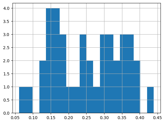
Since .summary() returns a pandas dataframe, you can use the “usual” pandas stuff for additonal analyses. For example, drawing a histogram of missing proportions:

p.summary().missing.hist(bins=20)

<Axes: >

_images/f792df61c774791500634525fb3f93defdb933e88b22b561760663ff0417cda6.png

Interpolate Missing Values#

It may be desirable to interpolate these missing values to get more “complete” traces. But if there is too much missing data to be interpolated, the results might not be trustworthy. PupEyes supports linear or spline interpolation while setting the maximum proportion of missing values allowed for interpolation.

# linear interpolation (default) for trials with missing pct < 40%
p = p.interpolate(missing_threshold=0.4)

✓ Interpolation completed!
  → New column: 'pp_db_ar_xy_sm_it' (interpolated)
  → Previous column 'pp_db_ar_xy_sm' preserved.
  → 1 trial(s) failed.

   participant block  trial
0      sub001     A      6

Baseline Correction#

If you are interested in task-evoked pupillary responses, it is desirable to do baseline correction to get “cleaner” evoked responses. There are two ways to do baseline correction:

Subtractive: corrected size = pupil size - baseline
Divisive: correct size = pupil size / baseline

There is a compelling argument to avoid divisive baseline correction due to its proneness to producing outliers. PupEyes by default uses the subtractive method.

PupEyes assumes that the baseline data is in the same dataframe as the to-be-corrected data. In our example, the baseline period consists of gaze samples occurred during the fixation period.

We will set the baseline data to the "fixation" period and use the mean of the last 100 samples for the actual correction on each trial.

p = p.baseline_correction(baseline_query='event=="fixation"', baseline_range=[-100, None])

✓ Baseline correction completed!
  → New column: 'pp_db_ar_xy_sm_it_bc' (baseline corrected)
  → Previous column 'pp_db_ar_xy_sm_it' preserved.
  → 1 trial(s) failed.

   participant block  trial
0      sub001     A      6

Note

The query string for baseline_query is used in the .query() method in pandas, see: https://pandas.pydata.org/docs/reference/api/pandas.DataFrame.query.html
The list-slicing syntax for the baseline_range argument makes it easy to specify different ranges of baseline data. E.g., [None, None] to use all baseline data, [-100, None] to use the last 100 samples, [None, 100] to use the first 100 samples, etc.

Now we have performed a series of preprocessing steps. PupEyes adds a new column with a suffix for each preprocessing step to preserve existing data:

_db: Deblink
_ar: Artifact rejection
_xy: Filter gaze position
_sm: Smoothing
_it: Interpolation
_bc: Baseline correction

p.data.head(5)

	participant	block	trial	event	trialtime	pp_db	pp_db_ar	pp_db_ar_xy	pp_db_ar_xy_sm	pp_db_ar_xy_sm_it	pp_db_ar_xy_sm_it_bc
0	sub004	A	1	fixation	0	<NA>	<NA>	<NA>	<NA>	5670.567834	550.902786
1	sub004	A	1	fixation	1	<NA>	<NA>	<NA>	<NA>	5670.567834	550.902786
2	sub004	A	1	fixation	2	<NA>	<NA>	<NA>	<NA>	5670.567834	550.902786
3	sub004	A	1	fixation	3	<NA>	<NA>	<NA>	<NA>	5670.567834	550.902786
4	sub004	A	1	fixation	4	<NA>	<NA>	<NA>	<NA>	5670.567834	550.902786

Chained Operations#

The above operations can be chained together as a complete processing pipeline.

p = pe.PupilProcessor(
    data=samples,
    trial_identifier=['participant', 'block', 'trial'],
    x_col = 'x',
    y_col = 'y',
    pupil_col = 'pp',
    time_col = 'trialtime',
    samp_freq = 1000,
    convert_pupil_size=False,
    progress_bar=True
    )\
    .deblink()\
    .artifact_rejection()\
    .filter_position(vertices=vertices)\
    .smooth()\
    .check_missing()\
    .interpolate(missing_threshold=.4)\
    .baseline_correction(baseline_query='event=="fixation"', baseline_range=[-100, None])

Device: eyelink
Eye-tracker missing value for pupil size is 0. No replacement needed.

Sampling frequency check passed. Sampling rate: 1000Hz
PupilProcessor initialized with 679965 samples
Pupil column: pp, Time column: trialtime, X column: x, Y column: y
Trial identifier: ['participant', 'block', 'trial'], Number of trials: 40
Running deblink using sampling frequency 1000Hz

✓ Deblinking completed!
  → New column: 'pp_db' (blinks removed)
  → Previous column 'pp' preserved.
  → 0 trial(s) failed.

✓ Artifact rejection completed!
  → New column: 'pp_db_ar' (artifacts removed)
  → Previous column 'pp_db' preserved.
  → 0 trial(s) failed.

✓ Gaze spatial filtering completed!
  → New column: 'pp_db_ar_xy' (gaze filtered)
  → Previous column 'pp_db_ar' preserved.
  → 0 trial(s) failed.

✓ Smoothing completed!
  → New column: 'pp_db_ar_xy_sm' (smoothed)
  → Previous column 'pp_db_ar_xy' preserved.
  → 0 trial(s) failed.

✓ Missing values checked!
  → 0 trial(s) failed.

✓ Interpolation completed!
  → New column: 'pp_db_ar_xy_sm_it' (interpolated)
  → Previous column 'pp_db_ar_xy_sm' preserved.
  → 1 trial(s) failed.

   participant block  trial
0      sub001     A      6

✓ Baseline correction completed!
  → New column: 'pp_db_ar_xy_sm_it_bc' (baseline corrected)
  → Previous column 'pp_db_ar_xy_sm_it' preserved.
  → 1 trial(s) failed.

   participant block  trial
0      sub001     A      6

PupilViewer: Interactive App for Inspecting Pupil Traces#

It is critical to use the PupilViewer to examine the quality of preprocessing. PupilViewer is built on Plotly Dash, an interactive web-based library for data visualization.

With PupilViewer, you can check if operations like deblinking, interpolation, and baseline correction are done properly.

To launch PupilViewer, create an instance by passing your PupilProcessor object to PupilViewer and call run(). Use the dropdown menus to select which trial and columns to plot.

You can hover over data points, drag, use the toolbar to zoom in/out, and more. Below is a screenshot of running it on my machine.

viewer = pe.PupilViewer(p, hue='event')

#viewer.run()

Tip

You can adjust how the app is run, such as whether it runs inline or in another tab, window size, etc., by passing keyword arguments to run_server(). See https://dash.plotly.com/dash-in-jupyter

Diagnostic Plots#

In addition to PupilViewer, PupEyes provides three interactive diagnostic plots to examine outlier data.

Gaze Position#

As much as we want participants’ eyes to stay still, we can never completely avoid the pupil foreshortening error. Sometimes, participants drift away from the screen center, either intentionally or unintentionally. Other times, though, the experimenter may display stimuli that encourage eye movements (such as a picture). In these cases, we have to make sure that gaze positions do not confound with the experimental variable we are interested in.

The plot_pupil_surface() function visualizes the extent of gaze spread, which may help you determine the extent of pupil foreshortening error. In the example below, we plot a 2D histogram of pupil size measurements as a function of their gaze coordinates. The red cross shows the average gaze position.

Note that here we do not have a condition variable, so we will just use participant instead. This will visualize if different participants fixated at different positions.

p.plot_pupil_surface(
    pupil_col='pp_db_ar_xy', # the remaining pupil measurements right after the gaze filtering step
    plot_by='participant', # here we plot by participant but you can also plot by an experimental condition if you like
    vertices=vertices, # you can optionally pass a region you used for filtering
    show_centroid=True # use False if it blocks data
)

As can be seen from this plot, our participants seemed to follow our instructions pretty well: they were fixating on the screen center most of the time.

plot_pupil_surface() is meant to provide a visualization only and doesn’t give you a statistical test of positional biases. However, if you include filter_position() in your preprocessing pipeline, you can see avg_gaze_x and avg_gaze_y columns in the summary data. These are the average gaze position for the remaining samples (i.e., after spatial filtering) for each trial. This information might be useful for additional analyses on gaze positions.

gaze_info = p.summary()[['participant','block','trial','run_gaze_filter','pct_gaze_filter','avg_gaze_x','avg_gaze_y']]
gaze_info.head(5)

	participant	block	trial	run_gaze_filter	pct_gaze_filter	avg_gaze_x	avg_gaze_y
0	sub004	A	1	True	0.001298	932.023893	592.014834
1	sub004	A	2	True	0.03203	975.807543	604.144581
2	sub004	A	3	True	0.018775	955.872528	597.951776
3	sub004	A	4	True	0.066141	954.471826	580.816997
4	sub004	A	5	True	0.022356	942.64441	585.789132

For example, we can compute the average gaze position for each participant and block:

# compute the mean gaze after filtering for each participant
gaze_info.groupby(['participant','block'])[['avg_gaze_x','avg_gaze_y']].mean()

		avg_gaze_x	avg_gaze_y
participant	block
sub001	A	858.581525	505.699754
sub002	A	976.501251	528.794445
sub003	A	972.302633	543.972819
sub004	A	946.053655	590.897507

If there are systematic biases in gaze position exist in your data, you might want to remove certain subjects/blocks/trials, or use a smaller region for filter_position().

Extreme Baseline Values#

Recall that we specified the last 100 samples of the fixation period as our baseline data. Well, what if some of these baseline pupil size values were distorted somehow? PupEyes provides a check_baseline_outliers method to detect baseline outliers. The outlier threshold is set as a constant n_mad_baseline* MAD.

You can optionally do the outlier detection by group.

p = p.check_baseline_outliers(
    n_mad_baseline=4, # larger values mean wider thresholds
    outlier_by='participant', # do outlier detection by participant
)

✓ Baseline outlier detection completed!
  → 3 trial(s) detected as baseline outliers.

    participant block  trial
20      sub002     A      1
32      sub001     A      3
37      sub001     A      8

Outlier Traces#

Another useful visualization is to plot the pupil size traces in one spaghetti plot. Mathôt and Vilotijević (2022) says that

Good-quality data will look like a tangle of lines.

A key sign of poor data quality is the presence of spikes that shoot downwards (but rarely upwards) from this tangle of lines: these spikes correspond to blinks or other recording artifacts that were not successfully interpolated or removed.

Another sign of poor data quality is the presence of lines that are far above (but rarely below) the others, or that start from zero but then quickly (< 200 ms) shoot upwards: these lines correspond to trials on which there were artifacts during the baseline period, resulting in extremely small baseline pupil sizes (which should also be evident in the histogram of baseline pupil sizes) and thus extremely large baseline-corrected pupil sizes.

PupEyes identifies outlier traces by comparing the max and min values of individual traces against an outlier threshold. This threshold is defined as a constant n_mad_trace * the MAD of max trace deviations from the overall mean. The default n_mad_trace is set to 4. If, at any point, a pupil trace crosses that threshold, it is marked as an outlier trace.

Select sub004 from the dropdown menu to inspect the detected outlier trace.

p = p.check_trace_outliers(
    pupil_col = 'pp_db_ar_xy_sm_it_bc', # which pupil column?
    n_mad_trace=3, # larger values mean wider thresholds; setting to 3 here to get an outlier trace as example
    outlier_by= 'participant' # do outlier detection by participant
)

Checking trace outliers for pp_db_ar_xy_sm_it_bc

✓ Trace outlier detection completed!
  → 1 trial(s) detected as trace outliers.

   participant block  trial
1      sub004     A      2

Attention

Do not blindly follow outlier detection results, especially when using default values. These default values are arbitrary and may not be appropriate for your specific study. In the end, the researcher must carefully decide what constitutes an outlier for their own study.

Summary Data#

The .summary() method returns a pandas dataframe that shows a summary of the preprocessing steps:

p.summary().head(5) # showing the first 5 rows

	participant	block	trial	n_samples	run_deblink	pct_deblink	run_speed	pct_speed	run_size	...	run_interpolate	pct_interpolate	run_baseline_correction	baseline	baseline_outlier	baseline_upper	baseline_lower	trace_outlier	trace_upper	trace_lower
0	sub004	A	1	23115	True	0.042743	True	0.000692	True	...	True	0.061302	True	5119.665049	False	6171.273173	4460.529201	False	1300.677704	-1219.819811
1	sub004	A	2	23166	True	0.248468	True	0.001597	True	...	True	0.340456	True	4979.91167	False	6171.273173	4460.529201	True	1300.677704	-1219.819811
2	sub004	A	3	12197	True	0.169796	True	0.002378	True	...	True	0.250143	True	5547.351041	False	6171.273173	4460.529201	False	1300.677704	-1219.819811
3	sub004	A	4	10916	True	0.19705	True	0.002657	True	...	True	0.323837	True	6072.677204	False	6171.273173	4460.529201	False	1300.677704	-1219.819811
4	sub004	A	5	22768	True	0.157809	True	0.001976	True	...	True	0.251669	True	5971.157678	False	6171.273173	4460.529201	False	1300.677704	-1219.819811

5 rows × 27 columns

.summary() helps you develop a principled way of defining “bad” trials. For example, we mark any trial that has a failed processing step or is an outlier as a bad trial:

# get bad trials based on the summary data
p.bad_trials = p.summary().query('run_deblink==False | run_speed==False | run_size==False | run_gaze_filter==False | run_smooth==False | run_interpolate==False | run_baseline_correction==False | baseline_outlier==True | trace_outlier==True', engine='python')[['participant','block','trial']]
p.bad_trials

	participant	block	trial
1	sub004	A	2
20	sub002	A	1
32	sub001	A	3
35	sub001	A	6
37	sub001	A	8

You will notice that these “bad” trials consist of the one trial we did not interpolate (or baseline correct) due to high missingness, 3 trials with extreme baseline values, and 1 trial with outlier trace.

Tip

Above is just an example of defining bad trials. You can of course define alternative criteria for trial exclusion. For example, you can pass numeric criteria as a query string:

pct_deblink > .3 | pct_speed > .2 | pct_interpolate > .4

You can also manually specify trials to exclude:

# adding two more trials
more_bad_trials = pd.DataFrame([
    {'subject':'003', 'block':'A', 'trial':4},
    {'subject':'004', 'block':'A', 'trial':7},
    ])
p.all_bad_trials = pd.concat([p.bad_trials, more_bad_trials])

Validate Trials#

Once you have a final dataframe of bad trials, you can run the .validate_trials() method, which adds a new column to the data to indicate whether a given sample should be excluded. We simply pass the dataframe of bad trials as an argument:

p = p.validate_trials(p.bad_trials)

This add a Boolean column named valid to the pupil size data

p.data.head(5)

	participant	block	trial	event	trialtime	pp_db	pp_db_ar	pp_db_ar_xy	pp_db_ar_xy_sm	pp_db_ar_xy_sm_it	pp_db_ar_xy_sm_it_bc	valid
0	sub004	A	1	fixation	0	<NA>	<NA>	<NA>	<NA>	5670.567834	550.902786	True
1	sub004	A	1	fixation	1	<NA>	<NA>	<NA>	<NA>	5670.567834	550.902786	True
2	sub004	A	1	fixation	2	<NA>	<NA>	<NA>	<NA>	5670.567834	550.902786	True
3	sub004	A	1	fixation	3	<NA>	<NA>	<NA>	<NA>	5670.567834	550.902786	True
4	sub004	A	1	fixation	4	<NA>	<NA>	<NA>	<NA>	5670.567834	550.902786	True

…as well as the summary data.

p.summary().head(5)

	participant	block	trial	n_samples	run_deblink	pct_deblink	run_speed	pct_speed	run_size	...	pct_interpolate	run_baseline_correction	baseline	baseline_outlier	baseline_upper	baseline_lower	trace_outlier	trace_upper	trace_lower	valid
0	sub004	A	1	23115	True	0.042743	True	0.000692	True	...	0.061302	True	5119.665049	False	6171.273173	4460.529201	False	1300.677704	-1219.819811	True
1	sub004	A	2	23166	True	0.248468	True	0.001597	True	...	0.340456	True	4979.91167	False	6171.273173	4460.529201	True	1300.677704	-1219.819811	False
2	sub004	A	3	12197	True	0.169796	True	0.002378	True	...	0.250143	True	5547.351041	False	6171.273173	4460.529201	False	1300.677704	-1219.819811	True
3	sub004	A	4	10916	True	0.19705	True	0.002657	True	...	0.323837	True	6072.677204	False	6171.273173	4460.529201	False	1300.677704	-1219.819811	True
4	sub004	A	5	22768	True	0.157809	True	0.001976	True	...	0.251669	True	5971.157678	False	6171.273173	4460.529201	False	1300.677704	-1219.819811	True

5 rows × 28 columns

This makes excluding trials easy in subsequent data analysis, as now you have a single column indicating whether we should keep the data or not.

Customized Summary#

You can customize .summary() by:

Show a subset of columns.
Grouping by different levels (e.g., by subject or condition).
Specifying custom aggregation methods.

For example, summarizing at the level of subject may help you decide whether to remove certain participants or not.

# summary at participant level
p.summary(level='participant', agg_methods={'pct_deblink':'median','valid':'mean'})

	pct_deblink	valid
participant
sub001	0.127729	0.7
sub002	0.108811	0.9
sub003	0.244544	1.0
sub004	0.140929	0.9

Final Steps#

After preprocessing, you’ll typically want to prepare a final dataset for analysis. For example, you might want to:

Remove trials we marked as invalid
Rename the fully preprocessed pupil column to a shorter name
Remove unnecessary columns
Keep only data during stimulus presentation and remove baseline data (since we have already done baseline correction)
If we do the above, also reset the timestamp to stimulus onset
Merge information from another dataframe

None of these operations require PupEyes; You can do them via standard pandas operations.

# 1. Create a final dataset with only valid trials during stimulus presentation
p.final_data = p.data.query('valid==True & event=="stimulus"').reset_index(drop=True)

# 2. Rename the fully preprocessed pupil column to something more manageable
p.final_data['pp_final'] = p.final_data['pp_db_ar_xy_sm_it_bc']

# 3. Select only the relevant columns for analysis
p.final_data = p.final_data[[
    'participant',  # participant ID
    'block',        # block number
    'trial',        # trial number
    'event',        # event marker
    'trialtime',    # time relative to trial onset
    'x', 'y',       # gaze coordinates
    'pp_final'      # preprocessed pupil size
]]

# 4. Create a timestamp column indicating time since stimulus onset using pandas' groupby-transform routine
p.final_data['eventtime'] = p.final_data.groupby(['participant','block','trial']).trialtime.transform(lambda x: x - x.iloc[0]) # reset timestamp for each trial

# 5. Merge necessary information from another dataframe
# Here we assume a between-subject design
trial_info = pd.DataFrame(
    {'participant':['sub001','sub002','sub003','sub004'],
    'group':['A','A','B','B']}
)
p.final_data = p.final_data.merge(trial_info)

# Preview the data
p.final_data.head(5)

	participant	block	trial	event	trialtime	x	y	pp_final	eventtime	group
0	sub004	A	1	stimulus	983	867.3	572.7	-51.159402	0	B
1	sub004	A	1	stimulus	984	867.8	570.9	-51.729276	1	B
2	sub004	A	1	stimulus	985	868.2	569.1	-52.289048	2	B
3	sub004	A	1	stimulus	986	868.3	568.8	-52.839291	3	B
4	sub004	A	1	stimulus	987	867.7	569.7	-53.380616	4	B

Save Results#

Once you are done, you can save all your processing results in a single .pkl file for future use.

# p.save('myproject.pkl')

To load your saved object, simply do the following:

# p = pe.PupilProcessor.load('myproject.pkl')

If you just want to save/load the final data, you can do that via pandas since it’s just a dataframe:

# # save only the final data 
# p.final_data.to_csv('final_data.csv', index=False)

# # reload the data
# reloaded_data = pd.read_csv('final_data.csv')

Combining Multiple PupilProcessors#

Sometimes, it gets tricky to preprocess data for all participants in one PupilProcessor instance, either because of memory consumption or difficulty in inspecting the data. Another scenario is after you have preprocessed some data, a new batch of data comes in, and you don’t want to do the repetitive work. In these cases, you may end up having several PupilProcessor instances.

PupEyes allows you to combine these instances into a single instance as long as your preprocessing pipeline is identical across instances.

# Creating an exact copy
p2 = p.copy()
# combine two instances
p_combined = pe.PupilProcessor.combine([p, p2])

Pupil Preprocessing

Contents

Pupil Preprocessing#

Read Data#

Inititalize PupilProcessor#

Deblink#

Downsampling (Optional)#

Artifact Rejection#

Filter Gaze Positions#

Smooth Data#

Check Missing Data#

Interpolate Missing Values#

Baseline Correction#

Chained Operations#

PupilViewer: Interactive App for Inspecting Pupil Traces#

Diagnostic Plots#

Gaze Position#

Extreme Baseline Values#

Outlier Traces#

Summary Data#

Validate Trials#

Customized Summary#

Final Steps#

Save Results#

Combining Multiple PupilProcessors#